In the first part (What is a “Scanned Data” Utility, Anyhow) we learned about the concept of quickly and conveniently transcribing plot data into a tabular form with precision. In this second part we will examine the use of a recommended scanned data utility—Plot Digitizer by Joseph Huwaldt.
The first step in our examination of scanning graphics for tabular export is to obtain a bitmap image of the plot data. We are using the plot as released by On Semiconductor. This is easily found on the web but is included as a simple bitmap image with this tutorial.
Plot Digitizer may then be downloaded from SourceForget.net at:
https://sourceforge.net/projects/plotdigitizer/files/plotdigitizer/2.6.8/
This is merely an executable file which does not need to be installed. It will probably be most convenient for you to place it on your Windows desktop.
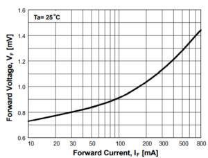 Invoke Plot Digitizer with the resulting window as shown in the illustration at right. To obtain your own do a google search using the terms “1n914 on semiconductor.” Download the 1n914 data sheet and find the plot in the document. Capture a bitmap image of it to a file.
It is now time to tell the application where to find the bitmap image which you just captured representing the plot data.
- Click File>Open…
- Navigate to the bitmap image file and click OK.
Make the plot fill up as much of the available space as is possible by “zooming.” Move the cursor to the upper banner of the application and hover around Zoom: and Out and In. Notice that as the cursor slides across Out and In that they highlight.
- Let the cursor rest on “In”
- Click
The magnification went from 100% to 150% and the plot filled a larger portion of the application window. Consider making the application footprint on the desktop larger and make the plot as large as possible but having the three corners still visible. This will help you with establishing the precise locations of the three corners.
The next step is to let Plot Digitizer know where the plot’s three corners are. Notice that Plot Digitizer is already suggesting to us the next step where it says at the bottom of the application:
Choose most negative end of the X axis
The idea is to identify the left-most corner of the X axis (which also happens to be a corner of the Y axis). Do that now. Notice that as you move the cursor around it is showing as a crosshair. Be slow and precise as you let the crosshair sit over the left-most X corner.
When the crosshair is precisely over the left-most X axis corner, click. The coordinates of that point are then identified and a dialog box appears as illustrated in Figure 3.
It is now time to identify the X axis value at that point. We can see that it is 10 mA but there is more to consider than its simple value. 10 mA is also 0.010 A. Which one should we use? The answer is that we can use either value as well as the silly value of 0.00001 kA. But the trick is that we have to from that point then be consistent in our naming convention.
Let’s consider advantages for using any of these values (let’s just skip consideration of 0.00001 kA, though). The advantage with using 10 mA is that the numbers are more readable. But the disadvantage is that the resulting table we produce will also be scaled in milli Amperes which may prove to be an inconvenience down the road depending on how we plan to use that table. When we consider using a scaling of Amperes we see that the readability is not all that bad, especially at the upper end of the scale where we have hundreds of milli Amperes. For this exercise will therefore us an Ampere scaling convention.
- In the “Value for X min” dialog box enter 0.01 but do NOT click Okay yet.
We now consider the axis scaling, whether it should be linear or logarithmic. Logarithmic axis scaling is particularly useful where magnitudes of numbers are being spanned such as micro Amperes to mega Amperes. But in this case our choice of axis scaling is preempted by the necessity to follow the convention of the plot. The plot convention is logarithmic.
- In the “Enter a Number” dialog box click the “Logarithmic Axis Scale box but to NOT yet click Okay.
The next consideration is what to do with the “Use X calibration for Y-axis” check box. Let’s leave this UN-checked.
And finally, it is virtually certain that you will always check the final box since for virtually all plots we are dealing with three corners as with this one.
- Click Okay.
Two things happen at that point. A “Enter a Number” dialog box appears asking what the Y-axis value is for this coordinate. Remember that this point serves as a corner for both the X and Y-axes.
Enter 0.6
Again, we must specify the axis to be either linear or logarithmic. The plot is linear so that is what we will use
- Leave UN-checked “Logarithmic Axis Scale
- Click Okay
Observe now that the messaging at the very most bottom of the application near the middle says, “Choose most positive end of X axis. Move the crosshair to superimpose over the far-right X-axis point.
- With the crosshair over the right X-axis point, mouse left click.
A dialog box similar to that of Figure 3 appears.
- Enter 0.8
- Click Okay
The message at the bottom of the application has changed once again. Now it says, “Choose most positive end of Y axis.”
- Move the crosshair to the far-left and far-highest point of the Y-axis and left-click.
A dialog box appears.
- Enter 1.6
- Click Okay.
It is now time to name the axes. A dialog box has appears asking for the name of the X axis. The x axis represents forward current.
- Enter “Amperes (A)”
- Click OK
A dialog box appears asking for the name of the Y axis.
- Enter “Voltage (V)”
- Click OK
Plot Digitizer now knows the coordinates defining the plot. Notice it has placed a red line over the X-axis and a blue line over the Y-axis. And notice a new message at the bottom of the application telling us to begin digitizeing points by clicking on the plot. But we must follow a protocol of moving only in one direction rather than picking coordinates randomly.
In this example we will start at the lowest current and work our way up. Click on the coordinate close to 0.01 Amperes, 0.72 Volts. But as you move the crosshair before you left-click, notice the two data windows at the far-left bottom of the application. As the crosshair moves these two windows identify the corresponding X,Y coordinates underneath the crosshair as it moves. Consequently, we can see that our eyeball estimate of that beginning coordinate representing 0.72 Volts is more precisely quantified as 0.7350 Volts.
- Left-click over the curve at 0.02 Amperes establishing a point there.
CAUTION: If you make a mistake and click somewhere you did not intend, do not try to move the data-point you just created. Do an undo and try again.
- Left-click over the curve at 0.03 Amperes. Recall that in part 1 this point looked like it fell precisely on the intersection of 0.03 A and 0.8 Volts. Low and behold, it digitizes to about that.
- Left click over the curve at 0.07 Amperes where we see a corresponding 0.869 Volts.
- Left-click over the curve at 0.09 Amperes.
- Then click on the Y-axis 1.0 Volts. Note that the corresponding current is about 0.170 Amperes.
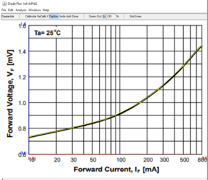 Pick a few more points until you have reached 0.80 Amperes. Also, you don’t need to place points on lines. Points can go where neither X nor Y line is found. When you are done your Plot Digitizer application will look something like that shown in the figure at right.
Let’s now save our work to disk.
- File>Export>Calibration & Data to XML.
- Pick a destination folder and file name and click SAVE.
Note that we do not save our work but export it.
In the next blog post we will look at importing our work back into the application and massage it for more precision using the aid of the application. We will then do an automatic generation of a tabular representation for this data.
Further, where these blogs are aimed is at device characterization for SPICE—Simulation Program with Integrated Circuit Emphasis. Ultimately we will be characterizing a 1N914 diode for use in a circuit that we simulate with SPICE. But the scanned data utility has usefulness way far and beyond any SPICE characterization.